C Additonal plotting tools
C.1 Plotting themes
Themes control non-data parts of your plots, such as:
- Overall appearance
- Axes
- Plot title
- Legends
They control the appearance of your plots (size, color, position) but not how the data is represented.
One example is theme_bw which provides a white background.
Other complete themes are: theme_classic, theme_minimal, theme_light, theme_dark.
More themes are available in the ggthemes package.
library(ggthemes)
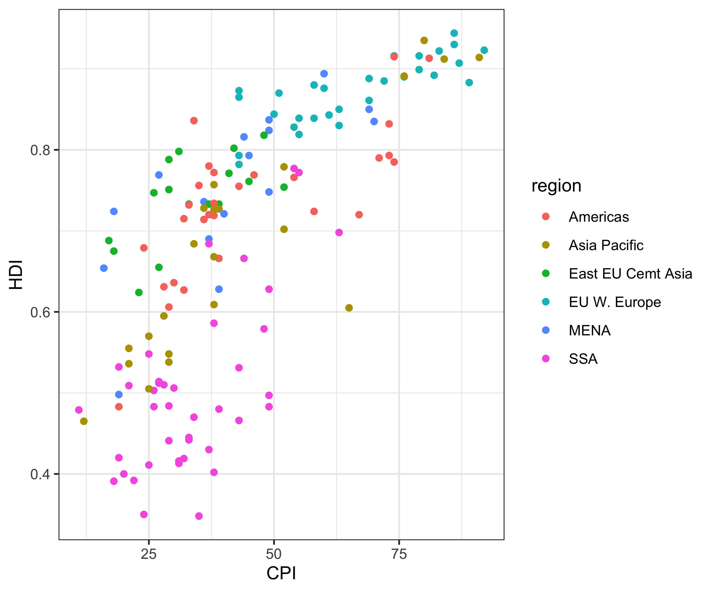
ggplot(ind, aes(CPI, HDI, color = region)) + geom_point() + theme_wsj() + scale_colour_wsj("colors6",
"")
Example of Wall Street Journal theme
C.2 Axes
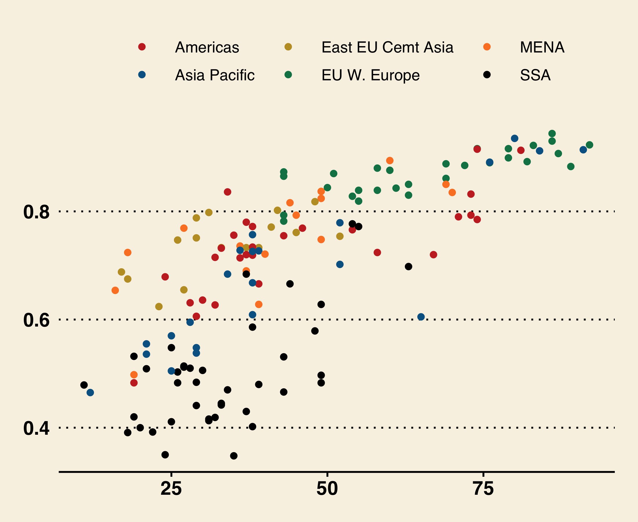
The appearance of the axis titles can be controlled with the global variable axis.title,
or independently for \(x\) and \(y\) using axis.title.x and axis.title.y.
ggplot(ind, aes(CPI, HDI, color = region)) + geom_jitter() + theme(axis.title = element_text(size = 20,
    color = "red"))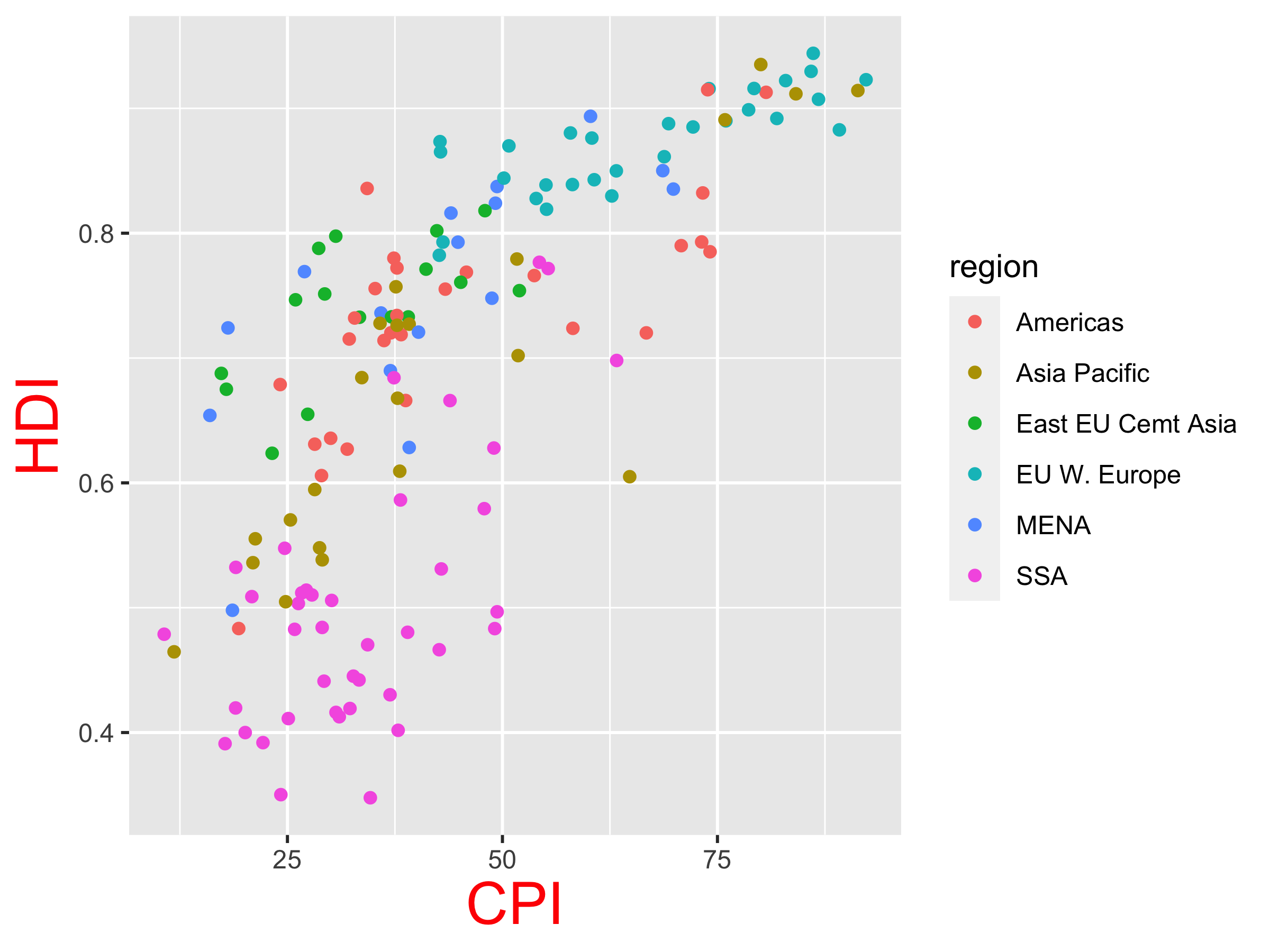
Similar for axis.text:
ggplot(ind, aes(CPI, HDI, color = region)) + geom_jitter() + theme(axis.text = element_text(size = 20,
    color = "blue"))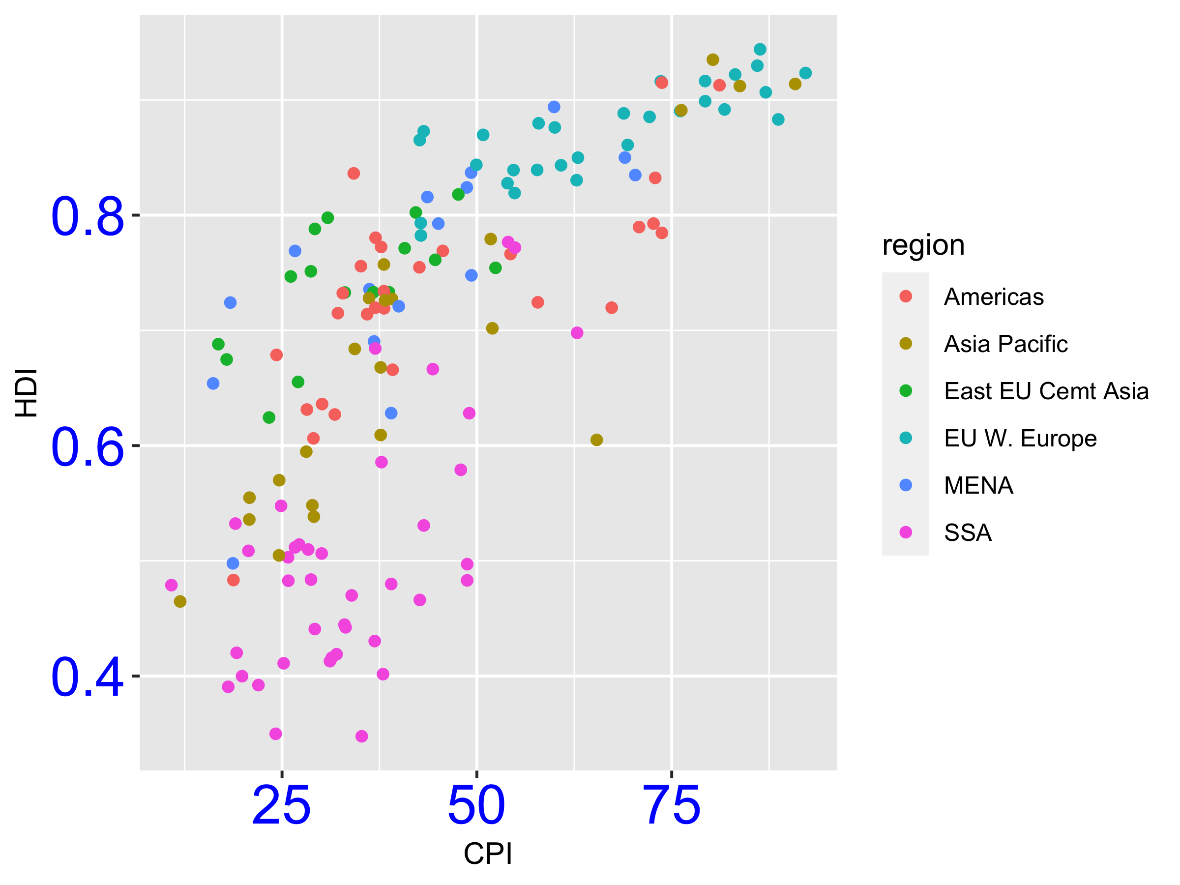
C.2.1 Axis elements
The axis elements control the appearance of the axes:
| Element | Setter | Description |
|---|---|---|
| axis.line | element_line() |
line parallel to axis (hidden in default themes) |
| axis.text | element_text() |
tick labels |
| axis.text.x | element_text() |
x-axis tick labels |
| axis.text.y | element_text() |
y-axis tick labels |
| axis.title | element_text() |
axis titles |
| axis.title.x | element_text() |
x-axis title |
| axis.title.y | element_text() |
y-axis title |
| axis.ticks | element_line() |
axis tick marks |
| axis.ticks.length | unit() |
length of tick marks |
C.3 Plot title
The appearance of the plot’s title can be controlled with the variable plot.title.
ggplot(ind, aes(CPI, HDI, color = region)) + geom_jitter() + ggtitle("CPI vs HDI") +
    theme(plot.title = element_text(size = 20, face = "bold"))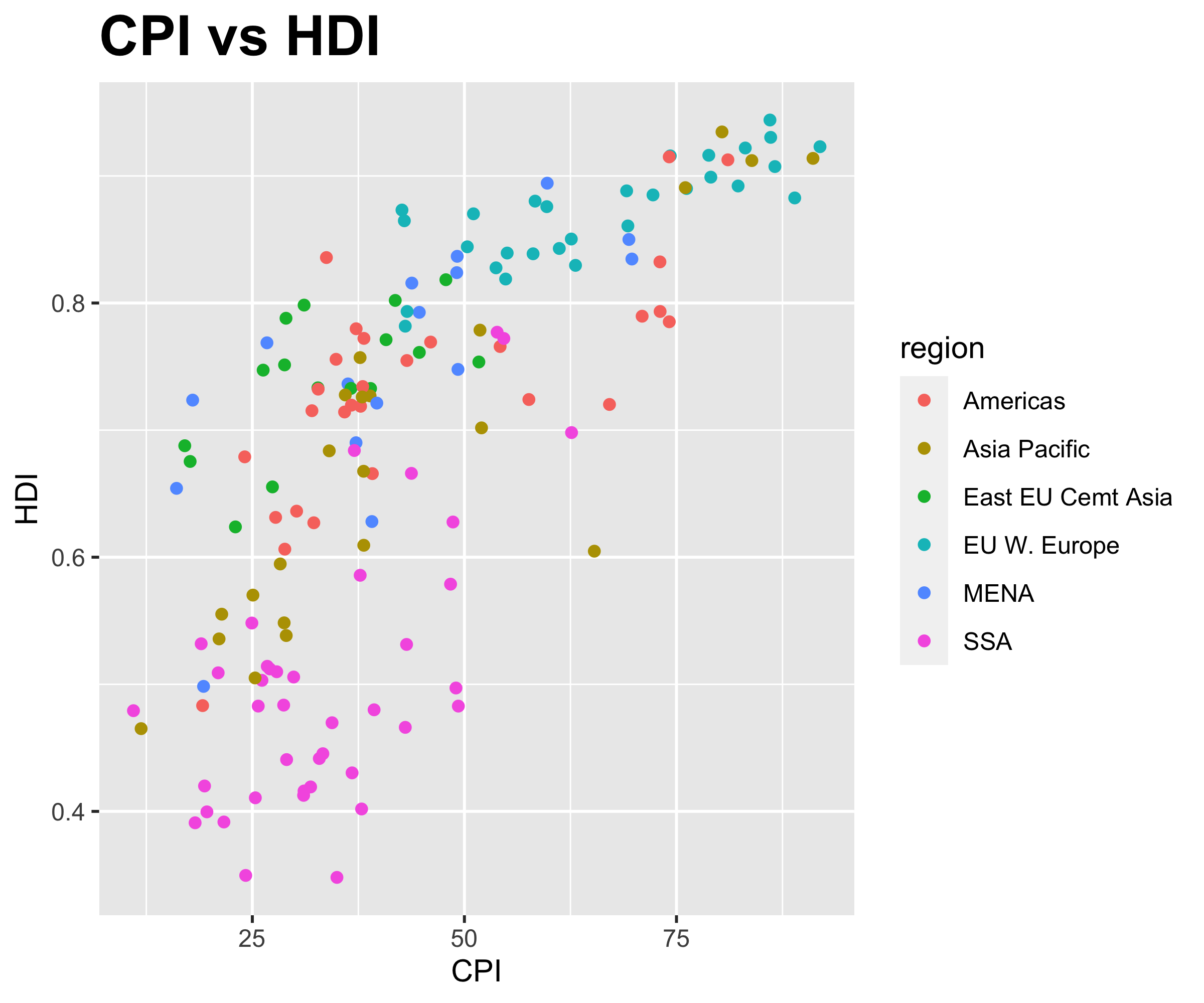
C.4 Legend
The appearance of the legend can be controlled with legend.text and legend.title.
base <- ggplot(ind, aes(CPI, HDI, color = region)) + geom_jitter()
base + theme(legend.text = element_text(size = 15), legend.title = element_text(size = 15,
    face = "bold"))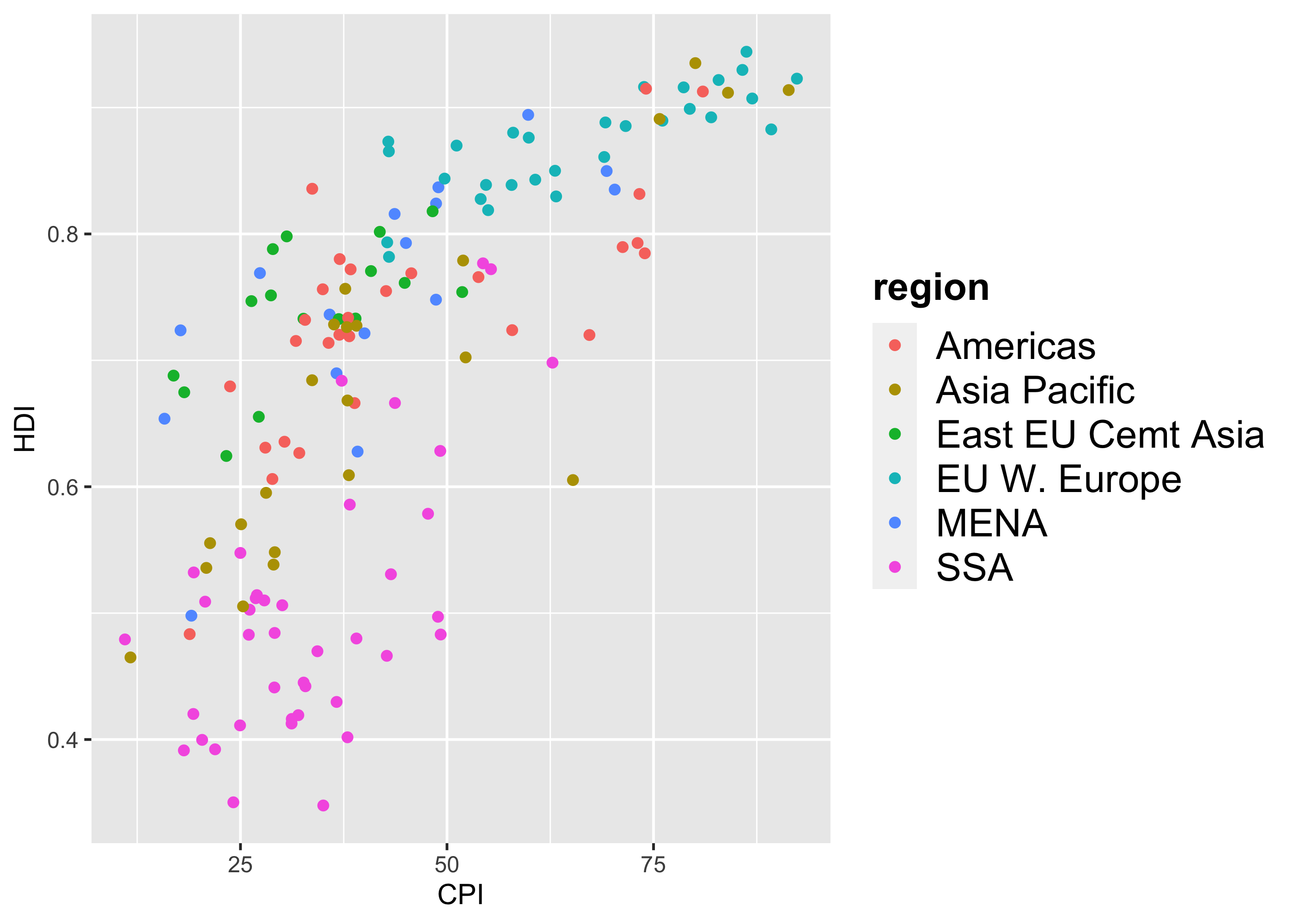
The legend elements control the appearance of all legends. You can also modify the appearance of individual legends by modifying the same elements in guide_legend() or guide_colourbar().
| Element | Setter | Description |
|---|---|---|
| legend.background | element_rect() |
legend background |
| legend.key | element_rect() |
background of legend keys |
| legend.key.size | unit() |
legend key size |
| legend.key.height | unit() |
legend key height |
| legend.key.width | unit() |
legend key width |
| legend.margin | unit() |
legend margin |
| legend.text | element_text() |
legend labels |
| legend.text.align | 0–1 | legend label alignment (0 = right, 1 = left) |
| legend.title | element_text() |
legend name |
| legend.title.align | 0–1 | legend name alignment (0 = right, 1 = left) |