B R programming

This Appendix covers the basic concepts of programming with R including control flow and functions. It is largely based on Rafael Irizzary’s book Introduction to Data Science [https://rafalab.github.io/dsbook/].

B.1 The pipe operator

The pipe operator, denoted %>% is a very convenient operator provided by the package magrittr. The pipe operator forwards a value, or the result of an expression, into the next function call or expression. The way to read an R line usiung the pipe operator is with the word “then”. For example, the following commands will complete exactly the same task:

library(magrittr)  # for pipe operator %>%

## First assignment without pipe operator
x <- 1000
log(x, 10)

## Second assignment with pipe operator Take x then compute log in base 10
x %>%
    log(10)

By default, the pipe operator forwards its left value into the first argument of the function call on its right. It is possible to specify another argument than the first one by using the . character.

## This computes log(x,10) Take x, then take the log in base 10
x %>%
    log(10)

## This too, where the base b=10 is forwarded to the second argument of log()
b <- 10
# Take b, then take the log of x in base b
b %>%
    log(x, .)

When performing several (nested) functions, the advantage of the pipe operator becomes particularly notable, since it allows clearer code readability and prevents bugs.

B.2 Conditional expressions

Conditional expressions are one of the basic features of programming. They are used for what is called flow control. The most common conditional expression is the if-else statement. In R, we can actually perform quite a bit of data analysis without conditionals. However, they do come up occasionally, and you will need them once you start writing your own functions and packages.

Here is a very simple example showing the general structure of an if-else statement. The basic idea is to print the reciprocal of a unless a is 0:

a <- 0

if (a != 0) {
    print(1/a)
} else {
    print("No reciprocal for 0.")
}

## [1] "No reciprocal for 0."

Let’s look at one more example using the US murders data frame:

library(dslabs)
data(murders)
murder_rate <- murders$total/murders$population * 1e+05

Here is a very simple example that tells us which states, if any, have a murder rate lower than 0.5 per 100,000. The if statement protects us from the case in which no state satisfies the condition.

ind <- which.min(murder_rate)

if (murder_rate[ind] < 0.5) {
    print(murders$state[ind])
} else {
    print("No state has murder rate that low")
}

## [1] "Vermont"

If we try it again with a rate of 0.25, we get a different answer:

if (murder_rate[ind] < 0.25) {
    print(murders$state[ind])
} else {
    print("No state has a murder rate that low.")
}

## [1] "No state has a murder rate that low."

A related function that is very useful is ifelse. This function takes three arguments: a logical and two possible answers. If the logical is TRUE, the value in the second argument is returned and if FALSE, the value in the third argument is returned. Here is an example:

a <- 0
ifelse(a > 0, 1/a, NA)

## [1] NA

The function is particularly useful because it works on vectors. It examines each entry of the logical vector and returns elements from the vector provided in the second argument, if the entry is TRUE, or elements from the vector provided in the third argument, if the entry is FALSE.

a <- c(0, 1, 2, -4, 5)
result <- ifelse(a > 0, 1/a, NA)

This table helps us see what happened:

a	is_a_positive	answer1	answer2	result
0	FALSE	Inf	NA	NA
1	TRUE	1.00	NA	1.0
2	TRUE	0.50	NA	0.5
-4	FALSE	-0.25	NA	NA
5	TRUE	0.20	NA	0.2

Here is an example of how this function can be readily used to replace all the missing values in a vector with zeros:

data(na_example)
no_nas <- ifelse(is.na(na_example), 0, na_example)
sum(is.na(no_nas))

## [1] 0

Two other useful functions are any and all. The any function takes a vector of logicals and returns TRUE if any of the entries is TRUE. The all function takes a vector of logicals and returns TRUE if all of the entries are TRUE. Here is an example:

z <- c(TRUE, TRUE, FALSE)
any(z)

## [1] TRUE

all(z)

## [1] FALSE

B.3 Defining functions

As you become more experienced, you will find yourself needing to perform the same operations over and over. A simple example is computing averages. We can compute the average of a vector x using the sum and length functions: sum(x)/length(x). Because we do this repeatedly, it is much more efficient to write a function that performs this operation. This particular operation is so common that someone already wrote the mean function and it is included in base R. However, you will encounter situations in which the function does not already exist, so R permits you to write your own. A simple version of a function that computes the average can be defined like this:

avg <- function(x) {
    s <- sum(x)
    n <- length(x)
    s/n
}

Now avg is a function that computes the mean:

x <- 1:100
identical(mean(x), avg(x))

## [1] TRUE

Notice that variables defined inside a function are not saved in the workspace. So while we use s and n when we call avg, the values are created and changed only during the call. Here is an illustrative example:

s <- 3
avg(1:10)

## [1] 5.5

## [1] 3

Note how s is still 3 after we call avg.

In general, functions are objects, so we assign them to variable names with <-. The function function tells R you are about to define a function. The general form of a function definition looks like this:

my_function <- function(VARIABLE_NAME) {
    # perform operations on VARIABLE_NAME and calculate VALUE
    VALUE
}

The functions you define can have multiple arguments as well as default values. For example, we can define a function that computes either the arithmetic or geometric average depending on a user defined variable like this:

avg <- function(x, arithmetic = TRUE) {
    n <- length(x)
    ifelse(arithmetic, sum(x)/n, prod(x)^(1/n))
}

We will learn more about how to create functions through experience as we face more complex tasks.

B.4 Namespaces

Once you start becoming more of an R expert user, you will likely need to load several add-on packages for some of your analysis. Once you start doing this, it is likely that two packages use the same name for two different functions. And often these functions do completely different things. Functions of different packages live in different namespaces. R will follow a certain order when searching for a function in these namespaces. You can see the order by typing:

search()

The first entry in this list is the global environment which includes all the objects you define.

If we want to be absolutely sure that R uses the function of specific package, we shall use double colons (::). For instance to force R to use the filter of the stats package, we can use

stats::filter

Also note that if we want to use a function in a package without loading the entire package, we can use the double colon as well.

For more on this more advanced topic we recommend the R packages book⁵⁴.

B.5 For-loops

The formula for the sum of the series \(1+2+\dots+n\) is \(n(n+1)/2\). What if we weren’t sure that was the right function? How could we check? Using what we learned about functions we can create one that computes the \(S_n\):

compute_s_n <- function(n) {
    x <- 1:n
    sum(x)
}

How can we compute \(S_n\) for various values of \(n\), say \(n=1,\dots,25\)? Do we write 25 lines of code calling compute_s_n? No, that is what for-loops are for in programming. In this case, we are performing exactly the same task over and over, and the only thing that is changing is the value of \(n\). For-loops let us define the range that our variable takes (in our example \(n=1,\dots,10\)), then change the value and evaluate expression as you loop.

Perhaps the simplest example of a for-loop is this useless piece of code:

for (i in 1:5) {
    print(i)
}

## [1] 1
## [1] 2
## [1] 3
## [1] 4
## [1] 5

Here is the for-loop we would write for our \(S_n\) example:

m <- 25
s_n <- vector(length = m)  # create an empty vector
for (n in 1:m) {
    s_n[n] <- compute_s_n(n)
}

In each iteration \(n=1\), \(n=2\), etc…, we compute \(S_n\) and store it in the \(n\)th entry of s_n.

Now we can create a plot to search for a pattern:

n <- 1:m
plot(n, s_n)

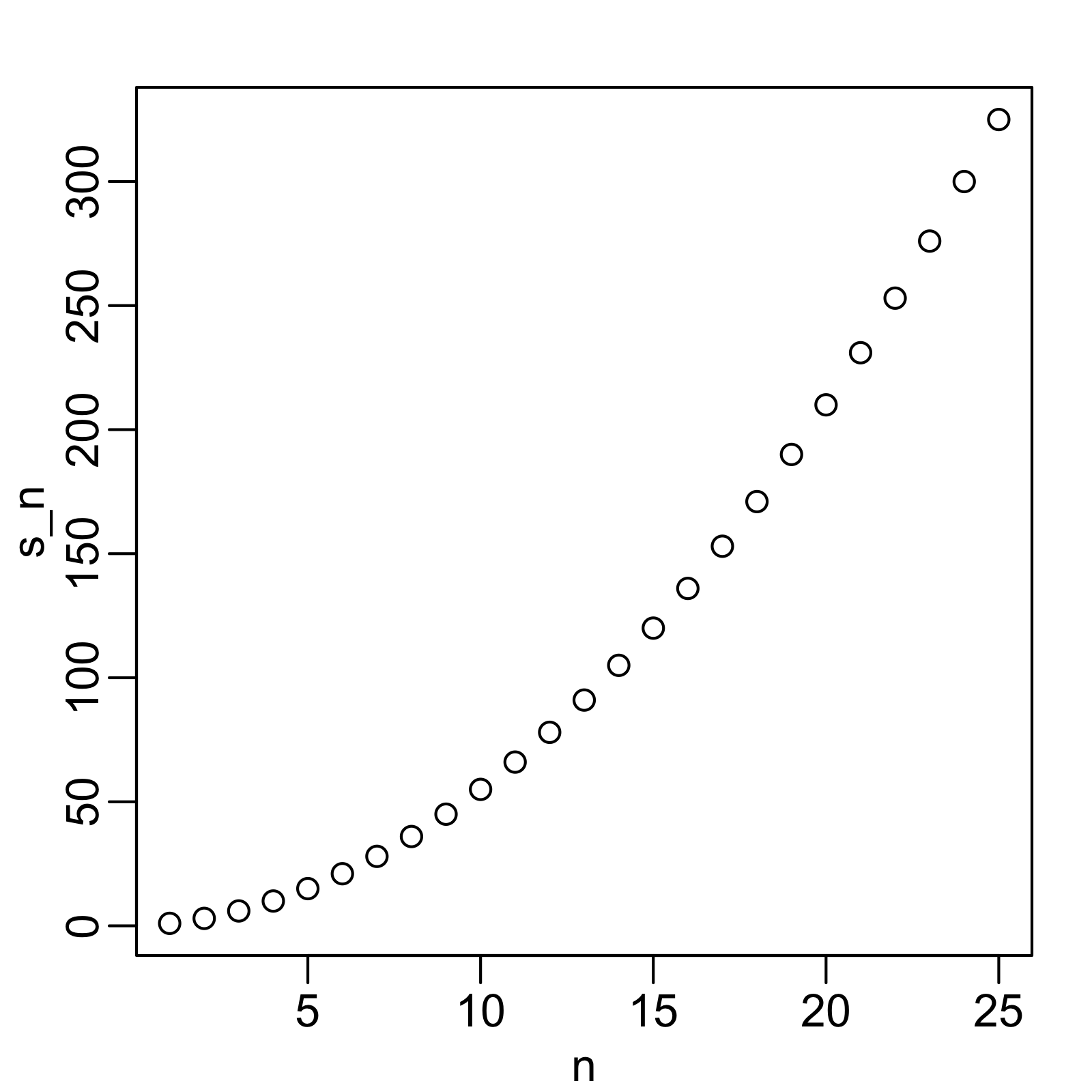
If you noticed that it appears to be a quadratic, you are on the right track because the formula is \(n(n+1)/2\).

B.6 Vectorization and functionals

Although for-loops are an important concept to understand, in R we rarely use them. As you learn more R, you will realize that vectorization is preferred over for-loops since it results in shorter and clearer code. We already saw examples in the Vector Arithmetic section. A vectorized function is a function that will apply the same operation on each of the vectors.

x <- 1:10
sqrt(x)

##  [1] 1.000000 1.414214 1.732051 2.000000 2.236068 2.449490 2.645751 2.828427
##  [9] 3.000000 3.162278

y <- 1:10
x * y

##  [1]   1   4   9  16  25  36  49  64  81 100

To make this calculation, there is no need for for-loops. However, not all functions work this way. For instance, the function we just wrote, compute_s_n, does not work element-wise since it is expecting a scalar. This piece of code does not run the function on each entry of n:

n <- 1:25
compute_s_n(n)

Functionals are functions that help us apply the same function to each entry in a vector, matrix, data frame, or list. Here we cover the functional that operates on numeric, logical, and character vectors: sapply.

The function sapply permits us to perform element-wise operations on any function. Here is how it works:

x <- 1:10
sapply(x, sqrt)

##  [1] 1.000000 1.414214 1.732051 2.000000 2.236068 2.449490 2.645751 2.828427
##  [9] 3.000000 3.162278

Each element of x is passed on to the function sqrt and the result is returned. These results are concatenated. In this case, the result is a vector of the same length as the original x. This implies that the for-loop above can be written as follows:

n <- 1:25
s_n <- sapply(n, compute_s_n)

Other functionals are apply, lapply, tapply, mapply, vapply, and replicate. We mostly use sapply, apply, and replicate in this book, but we recommend familiarizing yourselves with the others as they can be very useful.

B.7 R Markdown

This is an R Markdown presentation. Markdown is a simple formatting syntax for authoring HTML, PDF, and MS Word documents. For more details on using R Markdown see http://rmarkdown.rstudio.com.
Simply go to File –> New File –> R Markdown
Select PDF and you get a template.
You most likely won’t need more commands than in on the first page of this cheat sheet.
When you click the Knit button a document will be generated that includes both content as well as the output of any embedded R code chunks within the document.

B.8 Resources

Advanced R by Hadley Wickham Advanced R
In-depth documentations:
Last but not least:
- Stackoverflow

http://r-pkgs.had.co.nz/namespace.html ↩︎